Figure 1 of the paper, interactive. Moving the CV MAE from ImageNet to m-eurosat lifts its retention at its smallest budget (2.9% compute) from 10–33% to 74%, still below the 82–95% of RS FMs on the same dataset. Both the evaluation domain and RS-specific pretraining contribute.
Large-scale foundation models (FMs) in remote sensing (RS) are developed following paradigms established in computer vision (CV), yet the validity of transferring CV scaling laws to RS has not been systematically examined. We hypothesize that RS FMs enter an overparameterized regime at substantially smaller scales than their CV counterparts, with task-relevant information encoded redundantly across model dimensions.
To test this hypothesis, we apply post-hoc slimmability, uniform width reduction of pretrained encoder transformer blocks, as a tool to measure representational redundancy across ten state-of-the-art RS FMs on classification, segmentation, and change detection tasks. At their smallest compute budget (0.8–6.4% of full compute), most RS FMs retain more than 80% of their classification accuracy (85% on average), while MAE and DINOv2 pretrained on natural images retain only 10–33% on ImageNet subsets of matched class count at a comparable budget. A CV MAE evaluated directly on m-eurosat retains 74%, narrowing but not closing the gap to RS FMs on the same dataset (82–95%), indicating that both dataset characteristics and domain-specific pretraining contribute.
Mechanistic analyses such as feature correlation, explained variance, and effective dimensionality indicate that task-relevant variance concentrates in few principal components and is redundantly encoded across model dimensions. We further show that learned slimmable training improves over post-hoc slimmability for contrastive objectives, while reconstruction-based objectives do not benefit from current slimmable training protocols. Our findings establish post-hoc slimming as a practical deployment strategy for resource-constrained RS applications and as a diagnostic tool for representational redundancy in RS FMs.
RS FMs are highly slimmable. At their smallest compute budget, most models keep more than 80% of their full-scale accuracy on classification. Segmentation and change detection are even more robust.
The gap to CV is real, not an artefact of class count. CV MAE and DINOv2 collapse on ImageNet subsets with the same number of classes. On the same RS data, a CV MAE still degrades faster than RS FMs.
Smaller can be better. Intermediate widths often match or beat the full model, consistent with redundant dimensions acting as noise for the task.
Learned slimming helps contrastive, not reconstructive, pretraining. Slimmable MoCo improves at low budgets; slimmable MAE does not benefit under current protocols.
Redundancy is visible in the features. Slimmed representations concentrate variance in few, highly correlated directions, and this suffices for the downstream task.
Post-hoc slimming: one knob, no retraining
We take a released checkpoint and keep only a fraction s of the hidden width in every block: the first ⌊s·dk⌋ dimensions of each attention head and the first ⌊s·dh⌋ units of each feed-forward layer. The method is deliberately simple. If a sophisticated compression method preserved accuracy, it would be unclear whether that reflects the method or the model. If naive slimming preserves accuracy, it tells us something about the model.
with \(d_h' = \max(1, \lfloor s\cdot d_h \rfloor)\), \(s\in(0,1]\).
\(\mathbf{Q},\mathbf{K},\mathbf{V}\) use rows \(\mathcal{I}\) of their projections, the output projection uses columns \(\mathcal{I}\). All \(H\) heads are kept.
Frozen features, 31 widths
k-NN (k = 5) or linear probe on penultimate features for classification; a SegFormer-style multi-scale head for segmentation and change detection. Five seeds for classification; one run per width for segmentation and change detection.
Relative compute and retention
Compute = FLOPs at width s / FLOPs at full width. Retention = metric(s) / metric(1.0), so datasets with different absolute scores are comparable.
GEO-Bench + OSCD
m-brick-kiln, m-eurosat, m-so2sat, m-bigearthnet (classification); m-cashew-plant, m-SA-crop-type (segmentation); OSCD (change detection).
Ten RS foundation models, seven datasets
DOFA, Prithvi-EO-2.0, TerraMind-1.0 (base and large each), SSL4EO ViT-S (DINO and MoCo), Panopticon and Copernicus-FM. Each line starts at that model's smallest reachable compute budget, which depends on how much of the model sits in the (unslimmed) patch embedding.
Task complexity sets the threshold: m-eurosat is stable down to the smallest budget, m-bigearthnet needs about 2–10% compute.
Segmentation and change detection are even more robust. On m-cashew-plant the curves are practically flat.
Larger variants degrade more smoothly. Prithvi holds up best at extreme slimming; DOFA shows the strongest non-monotonic peaks.
Does training for slimmability help?
We pretrain ViT-Base models from scratch with MoCo and with MAE, once regularly and once with slimmable training (full, minimal and three random widths per step, with distillation from the full network). Then we slim all four post hoc.
Explicit multi-width optimisation makes contrastive representations more robust to width reduction without sacrificing peak performance.
No established slimmable protocol exists for reconstruction objectives, and the contrastive recipe does not transfer. This remains an open problem.
Why does slimming work?
Three descriptive measures of the frozen features at each width. They give mechanistic intuition, not a causal proof.
Average absolute correlation between feature dimensions, over the strictly upper triangle of the correlation matrix (self-correlations excluded).
$$\mathrm{MFC}=\tfrac{2}{D(D-1)}\textstyle\sum_{i<j}\lvert\mathrm{corr}(\mathbf{e}_i,\mathbf{e}_j)\rvert$$High = dimensions are redundant copies of each other.
Share of variance per principal component of the mean-centred features. We report the slope of log EVR against log component index.
$$\mathrm{EVR}_i=\lambda_i\big/\textstyle\sum_j\lambda_j$$Steeper (more negative) = variance concentrated in fewer components.
Participation ratio of the covariance eigenvalues: how many dimensions carry independent variance.
$$d_{\text{eff}}=\big(\textstyle\sum_i\lambda_i\big)^2\big/\textstyle\sum_i\lambda_i^2$$Low = information lives in a few directions.

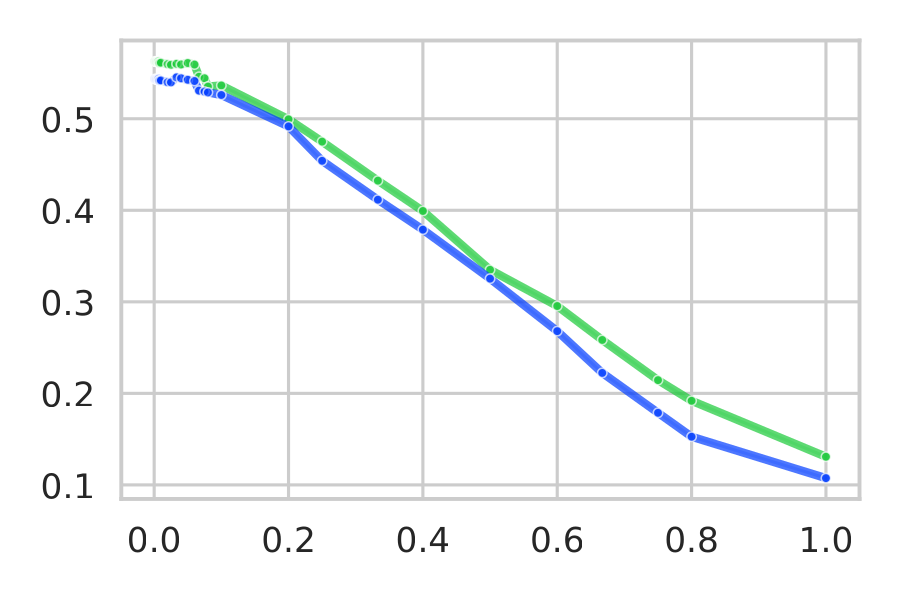
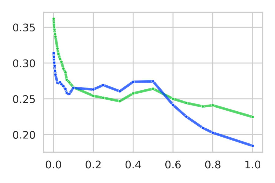
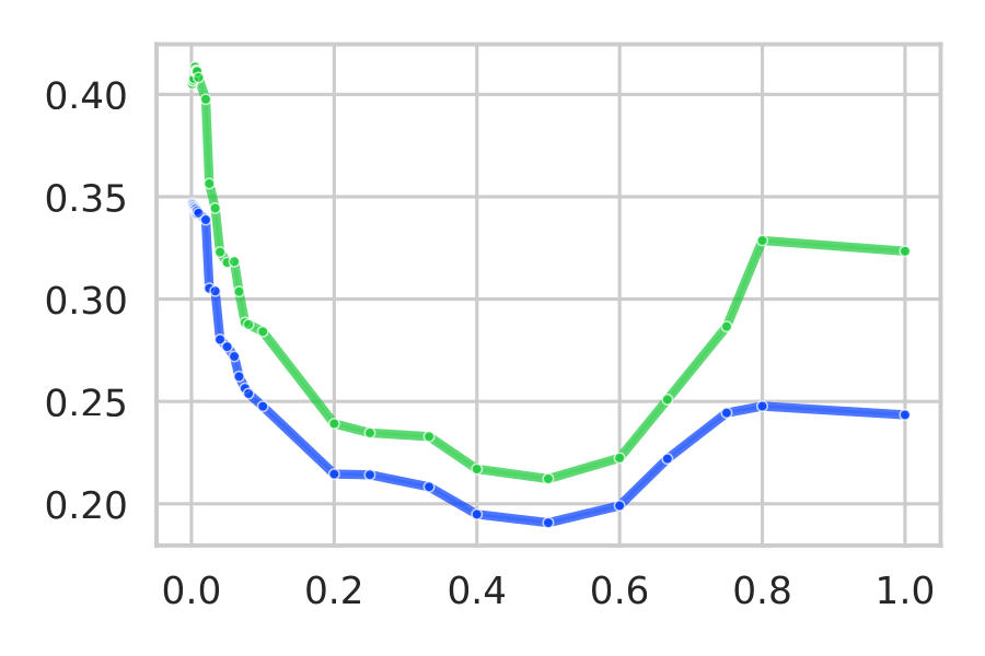
At the smallest budget, correlation is high for all three large models (≈0.56 for DOFA on m-eurosat) and falls as width grows.

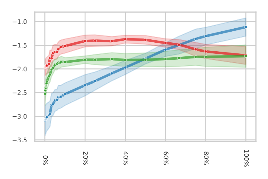
Log-log EVR slopes averaged over four classification datasets. DOFA steepens monotonically toward small widths (≈ −3.1); TerraMind stays flat until the smallest budget; Prithvi is non-monotonic.


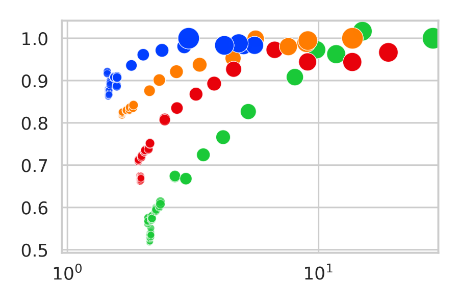
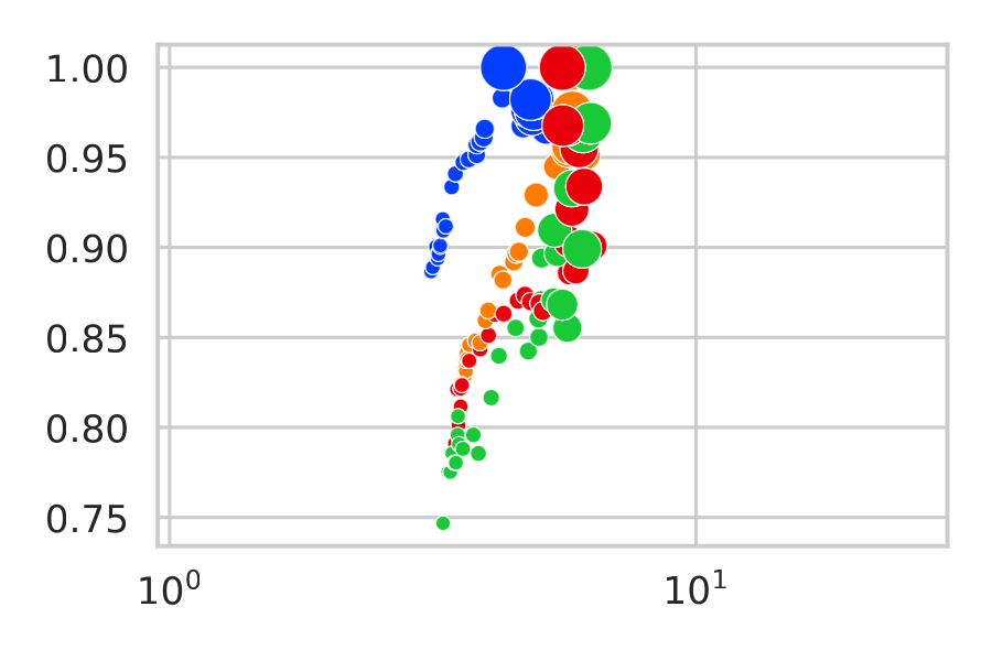
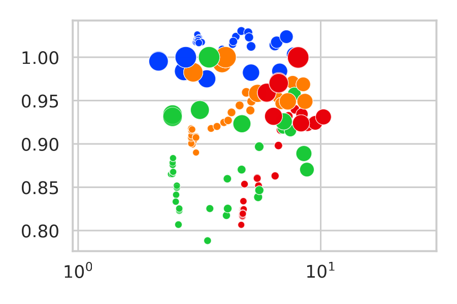
DOFA needs many independent dimensions at full scale (up to 34 on m-bigearthnet) and slimming removes them. Prithvi keeps 90–100% retention while its effective dimension varies by more than 2.5×.
DOFA (large): monotonic
TerraMind-1.0 (large): saturating
Prithvi-EO-2.0 (600M): decoupled
Is the redundancy an artefact?
We test whether the redundancy is an artefact of frozen features, model selection, geography or class balance.
Fine-tuning
Full fine-tuning (LR 3e-3, three seeds) raises absolute performance, but the accuracy-vs-width curves keep their shape. The redundancy is not an artefact of the frozen-feature protocol.
Panopticon · Copernicus-FM
Copernicus-FM is among the most slimmable models we evaluated. Panopticon is less slimmable but still substantially so. Note: Panopticon's embedding holds more than 66% of its parameters and is not slimmed, so its compute never drops below 63%.
m-so2sat
GEO-Bench's Cultural-10 split uses geographically disjoint train and test cities. A random split (five draws, same sizes) gives much higher retention, e.g. ≈0.93 vs ≈0.74 for DOFA (base) at the smallest budget. Distribution shift reduces redundancy, but a lot of it survives.
m-eurosat
Exponential class imbalance (class 0 keeps all samples, class 9 is subsampled down to the given ratio; five seeds). Accuracy drops at every width, but the curves stay roughly parallel: slimming does not interact strongly with imbalance.
m-bigearthnet
Hardest and easiest class per model (lowest / highest AP averaged over the five widths). Easy classes keep almost all their AP; the hardest lose a larger share than the aggregate mAP but do not fail outright. Aggregate metrics can hide uneven class-wise degradation.
Choosing a deployment width
With a labelled training set, pick the width by 5-fold cross-validation. Without one, label-space complexity, known in advance, is a reasonable first guess for where accuracy starts to fall off.
Why might RS FMs differ?
Three plausible, non-exclusive explanations. We did not test them directly.
Lower-level features suffice
Fewer nuisance factors
Benchmarks may be too easy
Scope and limitations
- Findings describe post-hoc width redundancy of the evaluated checkpoints, not a general scaling law for RS FMs.
- Read relative retention together with absolute performance, especially for safety-critical uses.
- Redundancy shrinks under geographic distribution shift, and aggregate metrics can mask class-wise degradation.
- All models are ViT-based and pretrained on optical Sentinel-2 data. SAR, CNN, hybrid, state-space and generative models (e.g. DiffusionSat) remain open.
- Complementary to scaling studies that pretrain one model per size (e.g. Dionelis et al., 2025): we ask how much of an already trained model is load-bearing.
Sanity checks from the appendix

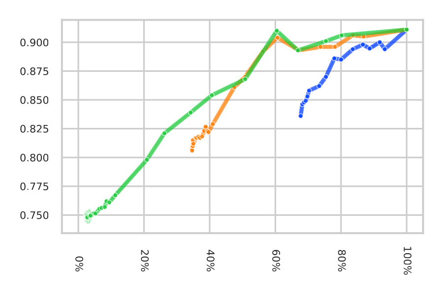
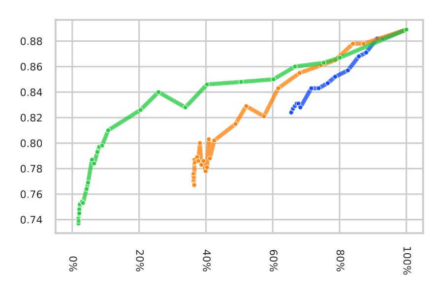
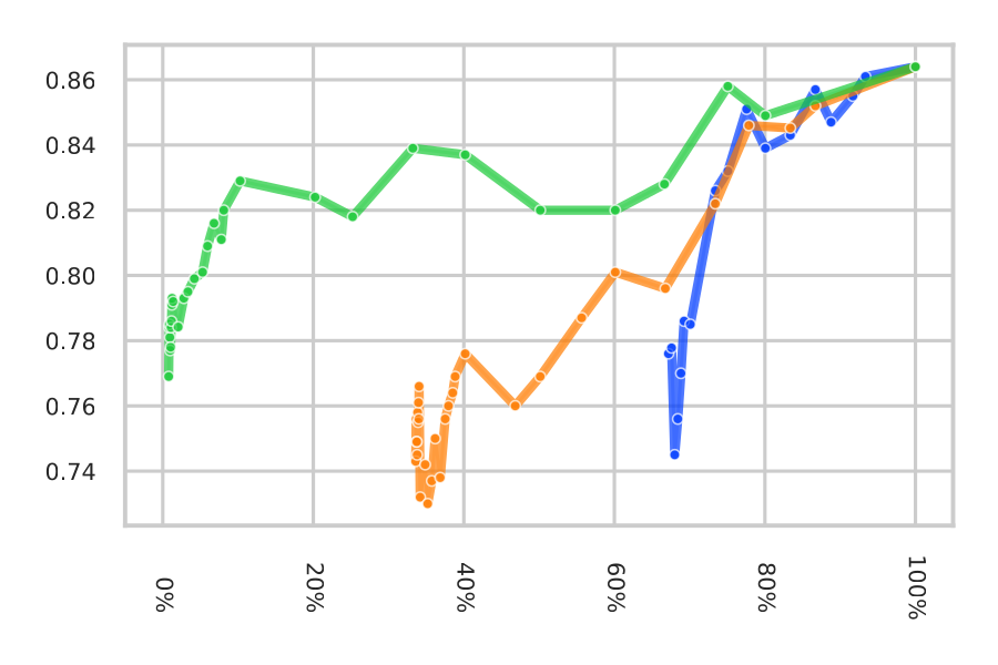
MHSA-only slimming cannot go below ≈65–69% compute; FFN-only reaches ≈34–37%. Slimming both jointly gives the best retention per FLOP and is the only way to reach the 0.8–6.4% range.

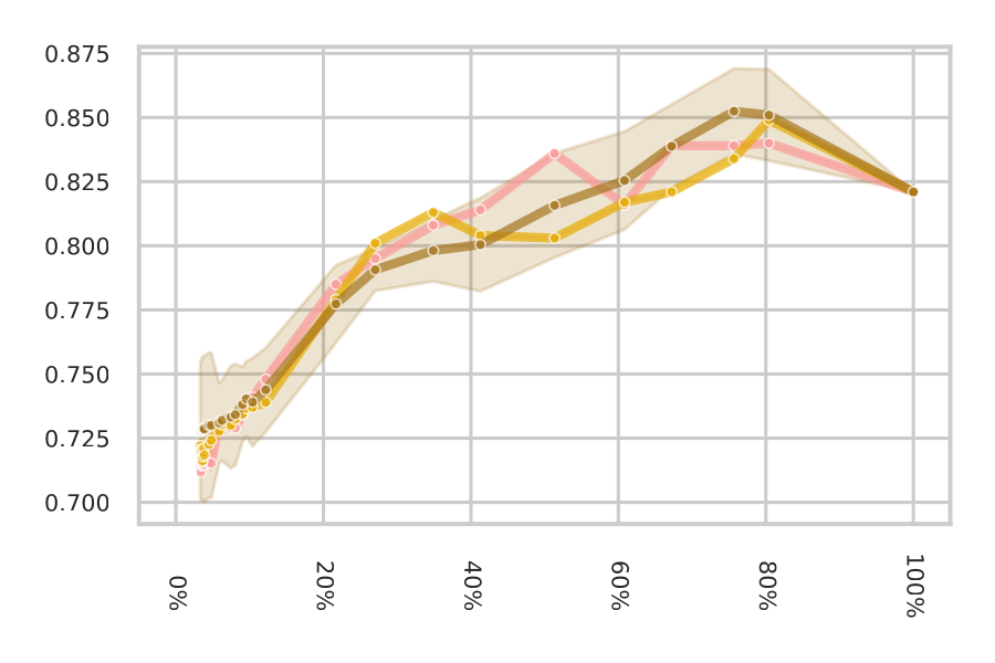
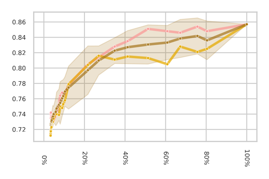
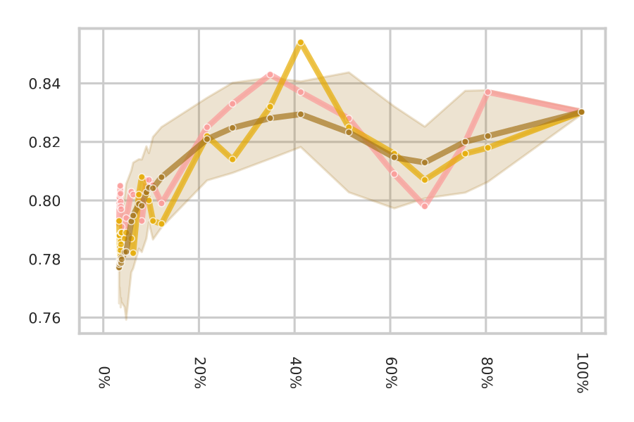
Keeping the first, last or a random subset of dimensions (20 draws, 2σ) gives comparable results: first/last never differ from the random mean by more than 2.8 accuracy points. A few widths fall outside the random 2σ band (e.g. DOFA “last” at 28–76% compute, Prithvi “first” below 1.6%), with no pattern shared across models.

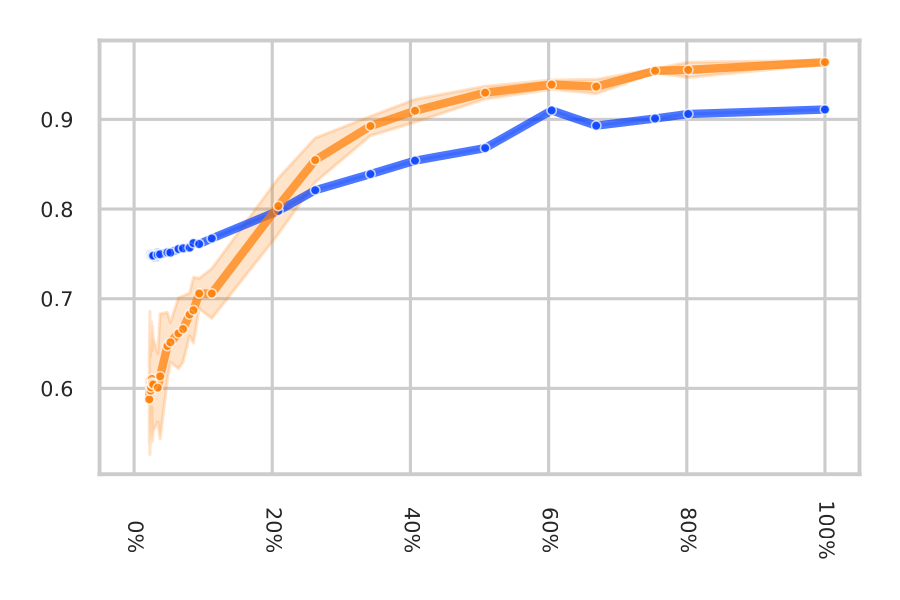
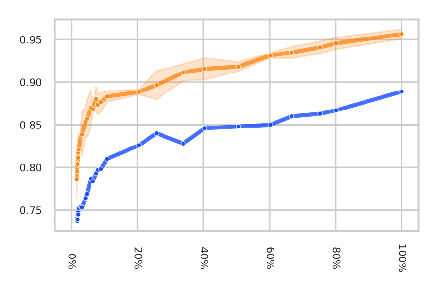
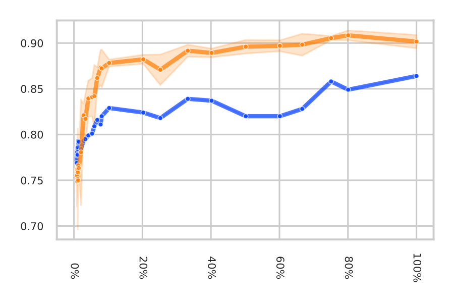
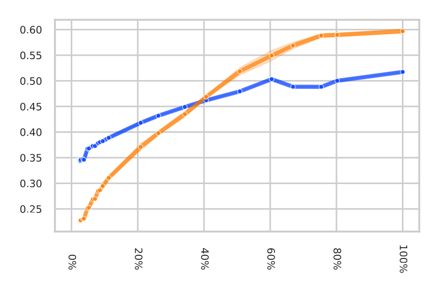
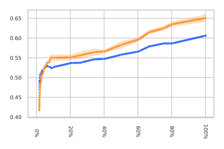
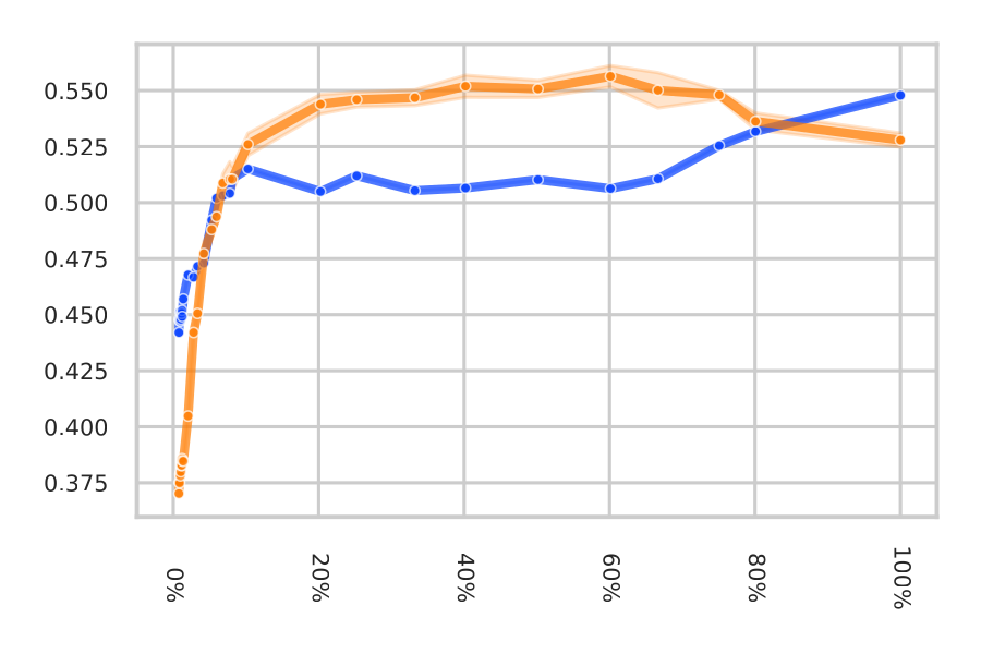
Linear probes win at large widths, k-NN tends to win for heavily slimmed models. The crossover width is not consistent across models or datasets.

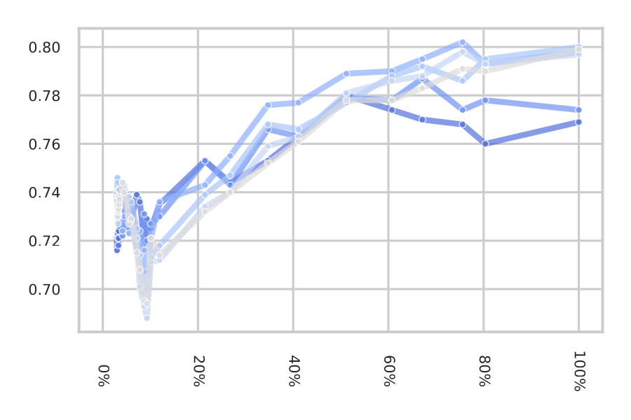
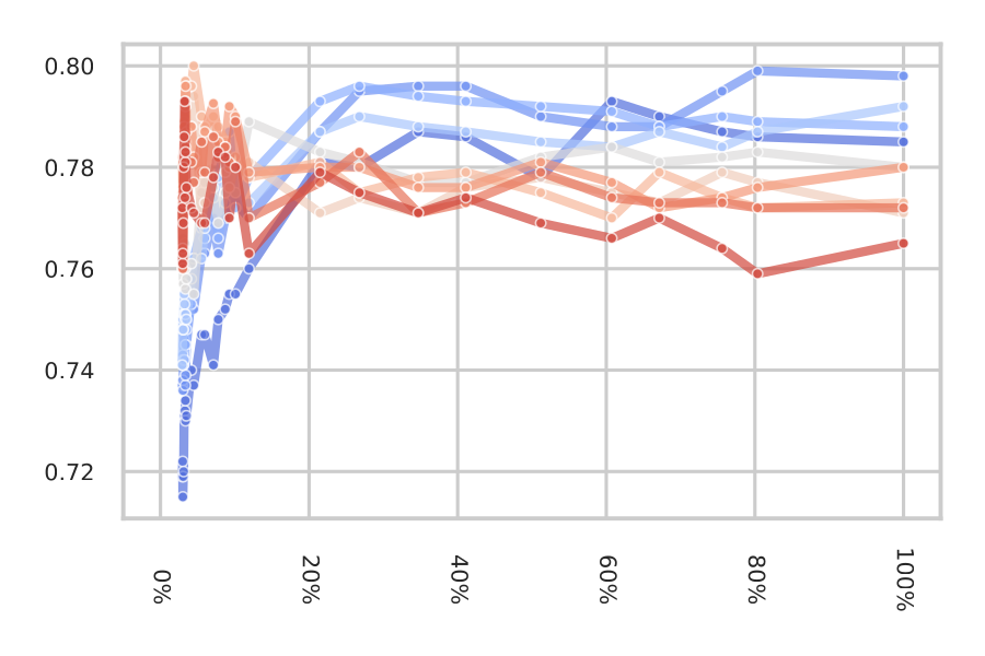
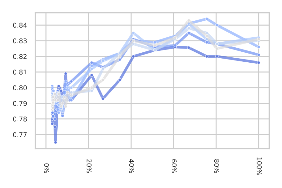
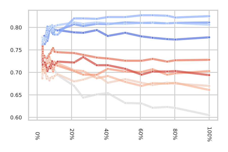
k-NN accuracy on m-eurosat at checkpoints during pretraining. Slimmable MAE improves for 200 epochs, then drops by almost 20% and never fully recovers. Slimmable MoCo equalises accuracy across widths with longer training.
Open code, pinned environment
All code for the experiments on this page will be released.
- MIT license.
- Pinned dependencies via Poetry's lockfile, plus the resolved environment specification.
- Checkpoint sources for every evaluated model.
- Fixed seeds: experiments with n runs use seeds {0, …, n−1}.
- CPU-friendly analysis: k-NN, EVR, correlation and effective dimension run on 16 CPU cores; feature extraction for all widths takes under 30 minutes per model.
# Illustration of the idea, not the released API
def slim_ffn(x, fc1, fc2, s):
    dh = max(1, int(s * fc1.out_features))
    h = act(x @ fc1.weight[:dh].T + fc1.bias[:dh])
    return h @ fc2.weight[:, :dh].T + fc2.bias

def slim_heads(W, b, H, dk, s):
    k = max(1, int(s * dk))
    idx = torch.cat([torch.arange(i*dk, i*dk + k) for i in range(H)])
    return W[idx], b[idx]   # rows for Q, K, V; columns for W_O
BibTeX
@inproceedings{hackel2026slimmable,
  title     = {How Much of a Model Do We Need? Redundancy and Slimmability
               in Remote Sensing Foundation Models},
  author    = {Hackel, Leonard and Burgert, Tom and Demir, Beg{\"u}m},
  booktitle = {Advances in Neural Information Processing Systems (NeurIPS)},
  year      = {2026}
}
This work is supported by the European Research Council Project Agent-BigEarth (No. 101292498) and the European Union Horizon Project PROTEUS (No. 101296397).